News
Proton Technology Developments
Announcing the Use of Geant4 to Obtain Crisp 3D pCT Images
Published 4/2026
Geant4 is widely regarded as the gold standard for simulating how protons traverse matter, particularly in the context of human patients. In this article, we present a method for reconstructing proton computed tomography (pCT) images using individual proton histories generated through Geant4 simulations.
We further demonstrate how these results represent a significant step toward the development of a clinically viable, commercial pCT system, highlighting both the underlying methodology and its practical implications for improving patient outcomes.
Introduction:
This article traces the workflow from simulation setup through pCT image reconstruction, providing a high-level view of the end-to-end process. It then examines the significance of this approach and its implications for the advancement of proton imaging technology.
The Raw Data:
On our website, we have outlined the data required to compute a proton computed tomography (pCT) image. To generate this data through simulation, the following workflow is implemented:
- Construct a slice composed of 1 mm³ voxels, each assigned a relative stopping power (RSP) corresponding to how much energy is deposited in a voxel by a proton of a given energy.
- Define the spatial and angular distribution of proton beams incident on the slice.
- Use a validated particle transport simulation tool, specifically Geant4, to determine the exit position and residual energy of each proton after traversing the slice.
- Process the raw simulation output to estimate the properties of an “ideal proton,” defined as one that travels along a straight path between its measured entry and exit points.
- Input the resulting idealized proton data into our proprietary pCT reconstruction algorithm.
- Compare and present the original (ground truth) slice, the reconstructed slice, and the voxel-wise differences between them.
This structured approach ensures a transparent link between simulation inputs, reconstruction methodology, and quantitative evaluation of image accuracy.
Step 1.
In our example case, the 30mm by 30mm by 1mm slice, was generated in Geant4 and a realistic RSP (see our website for an explanation of RSP) was assigned to each of the 900 voxels. This provides the ground truth mention above. We have also used CT scans to create human scale slices. However, the points we wish to illustrate are seen more clearly with smaller slices.

Figure 1. The ground truth slice as seen using MATLAB’s surface plot function. The color bar on the right indicates the RSP of each voxel. Note the RSP values correspond to how much energy 250MeV protons deposit in each voxel, assuming a path length in the voxel of 1mm.
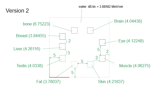
Figure 2. The same slice, showing the RSPs assigned to each voxel and the tissue equivalent of each RSP. Note all the tissue inserts are 9 voxels in size composed of 3 voxel by 3 voxel inserts. The green and red lines at the lower lefthand edge are used to indicate which is the row direction and which is the column direction.
In this case we choose Geant4 to simulate the slice as Geant4 is widely regarded as the gold standard for simulating how protons and other particles traverse matter, especially in complex, heterogeneous environments like the human body. Developed and maintained by an international collaboration led by CERN, Geant4 provides a comprehensive framework for modeling the full range of physical interactions that protons undergo, including electromagnetic energy loss, multiple Coulomb scattering, and hadronic (nuclear) processes. Its physics models are continuously validated against experimental data, ensuring that simulations closely reflect real-world behavior across a wide energy spectrum relevant to medical applications.
In the context of human patients, Geant4’s strength lies in its ability to accurately represent anatomical geometry and material composition at high resolution. Using voxelized patient data derived from CT scans, it can simulate proton transport through realistic tissue structures, accounting for variations in density and elemental composition that strongly influence proton range and scattering. As a result, Geant4 has become the benchmark tool for research and development in medical physics, enabling precise, physics-driven insights into how proton beams interact with the human body.
It is much faster than using the National Institute of Standards and Technology (NIST) PSTAR tables to construct slices. In routine workflows, we rely on the PSTAR tables for efficiency. However, for the purpose of demonstrating how raw data from individual protons is transformed into a crisp, accurate 3D image, we adopt the significantly slower Geant4 approach in this study. More details are provided below.
Step 2. The beam plan was entered into Geant4. This plan maximizes the amount of information obtained from each proton thus minimizing the dose to the patient. The beam plan tells the computer where to send the beams into the slice, at what energy, and what direction. Geant4 then uses the Monte Carlo simulation to track each proton of the beam as that proton transits the slices. Finally, it records where each proton exited, at what energy, and at what direction. The algorithm is only allowed to know this last information. We do not use the individual protons tracks, as that would not be known in a clinical setting.
Step 3. Geant4 then simulated the transit of proton beams (2,000 protons per beam) starting at the entrance points programed in Step 2. Note, in our commercial system, only some 200 protons per beam will be used to limit the patient’s absorbed dose. The higher number of protons per beam where used to confirm our Ideal Proton methodology mentioned below.
In the context of human patients, Geant4’s strength lies in its ability to accurately represent anatomical geometry and material composition at high resolution. Using voxelized patient data derived from CT scans, it can simulate proton transport through realistic tissue structures, accounting for variations in density and elemental composition that strongly influence proton range and scattering. This level of detail is essential for applications such as proton therapy and proton computed tomography, where even small inaccuracies in modeling can lead to clinically significant errors. As a result, Geant4 has become the benchmark tool for research and development in medical physics, enabling precise, physics-driven insights into how proton beams interact with the human body.
Step 3. Side Note
As noted above, we typically use the National Institute of Standards and Technology (NIST) PSTAR tables to construct image slices. Our proprietary algorithm does not rely on data from individual protons; instead, it employs a novel concept we refer to as Ideal Protons, described elsewhere on our website. A key advantage of this approach is that Ideal Protons can be computed directly from PSTAR data, enabling efficient reconstruction without detailed particle-by-particle simulation.
As a result, the use of Geant4 is only necessary in specific scenarios. These include evaluating how many individual protons are required to form a single Ideal Proton, assessing the impact of secondary particle production, and analyzing less common physical interactions such as Rutherford scattering. Additionally, Geant4 is used to study how simulation outputs depend on factors such as step size and transitions in material density.
Bottom of Form
Both National Institute of Standards and Technology NIST PSTAR tables and Geant4 provide reliable pathways for determining the residual energy of protons after they traverse a human patient, though they do so with different levels of complexity and fidelity. The NIST PSTAR tables offer tabulated stopping power and range data for protons in a variety of materials, including water, which is commonly used as a surrogate for human tissue. By integrating the stopping power along a known path length—or equivalently, by using water-equivalent path length (WEPL)—one can estimate how much energy a proton loses as it passes through the body and thus infer its exit energy. This approach is computationally efficient and widely used for analytical calculations, calibration, and validation tasks.
In contrast, Geant4 provides a fully stochastic, physics-based simulation of proton transport, capturing not only average energy loss but also fluctuations such as energy straggling, multiple scattering, and nuclear interactions. When applied to voxelized patient geometries derived from CT data, Geant4 can track individual proton histories and directly compute the distribution of exit energies after transit through heterogeneous tissues. While more computationally intensive than PSTAR-based methods, this approach offers significantly higher fidelity, particularly in situations where tissue composition varies or where secondary interactions play a non-negligible role. Together, these tools form complementary strategies: PSTAR tables enable fast, deterministic estimates, while Geant4 delivers detailed, high-accuracy predictions essential for advanced imaging and treatment planning.
Step 4.
Ideal Protons are constructed through a combination of selection and statistical interpretation. Specifically, we identify protons that travel close to a given straight-line path and analyze the distribution of their exit energies. From this distribution, we estimate a representative exit energy for that path—an approach that proves more straightforward than might initially be expected.
Importantly, no two protons following the same path will exit with identical energies. Simulations using Geant4 illustrate the extent of this variation. As a rule of thumb, the coefficient of variation for exit energy along a given path is approximately 0.6%. Consequently, estimating the exit energy to within about 6 parts in 1,000 is sufficient; attempting to measure the exit energy of an individual proton with higher precision offers no practical benefit.
In contrast, Ideal Proton exit energies are derived from ensembles of on the order of 100 individual protons, reducing the uncertainty to approximately 6 parts in 10,000 through statistical averaging. Because the number of Ideal Protons significantly exceeds the number of voxels in a proton computed tomography (pCT) reconstruction, the resulting uncertainty in relative stopping power (RSP) for each voxel is further reduced.

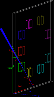
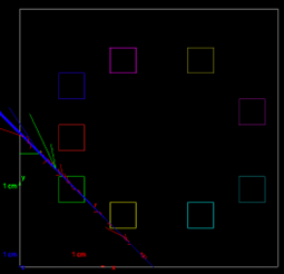
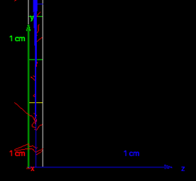
Figure 3. This figure, generated by Geant4, show the proton beam pattern running. Beams are sent in at points around the edge of the slice. The beam start at the middle of each edge voxel and are aimed at the middle of another edge voxel. The beams spread out due to Multiple Column Scattering (MCS). Geant4 outputs the position and energy of each proton in each beam.
As can be seen from figure 3, the spread of the beam is small compared to the number of protons sent in each direction. This makes estimating the average exit energy for each beam / Ideal Protons, straightforward.
Step 5.
As described elsewhere on our website, the Ideal Protons serve as inputs to the proton computed tomography (pCT) reconstruction algorithm. Our method employs an iterative, modified steepest descent method, which requires an initial estimate of the relative stopping powers (RSPs) for each voxel.
This initial guess is typically derived from uncertainties associated with Hounsfield units and their conversion to RSP. Alternatively, a uniform initialization—such as assigning all voxels the RSP of water—can be used. While this approach results in slower convergence, it does not affect the final accuracy of the reconstructed RSP values.
Step 6.
The algorithm seeks to minimize the difference between the measured exit energies and the exit energies as computed from the current estimated RSPs. The estimated RSPs are adjusted, step by step to find that set of RSPs which best minimizes the delta between computed and measured energy.

Figure 4. Best-fit reconstruction of the slice shown in Figure 1, rendered using the MATLAB surface plotting function. Careful examination reveals no visually discernible differences between Figures 1 and 4, aside from a slight change in viewing angle.
A better sense of the difference between the ground truth RSPs and the fit RSPs is given by the following histogram.
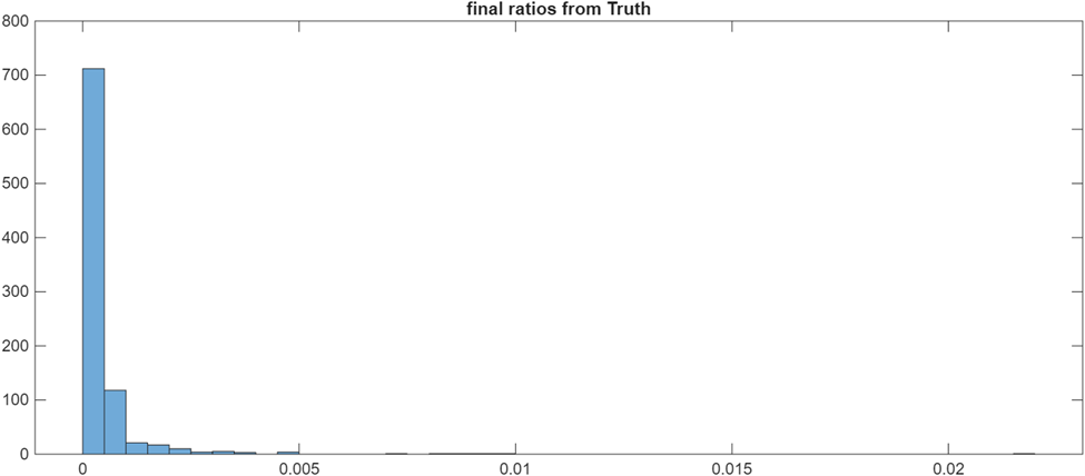
Figure 5. Histogram of the fractional differences between the true relative stopping powers (RSPs) and the fitted RSPs. The x-axis represents the ratio for each voxel, defined as (true RSP – fitted RSP) / true RSP. The y-axis shows the number of voxels whose ratios fall within each bin.
Notably, nearly all of the 900 voxels are reconstructed with fractional differences below 0.005. The small number of voxels that fall outside this range are discussed below.
The quality of the fit is evident in Figure 5; however, it does not represent the best achievable result. The observed discrepancies arise primarily from the transition between using Geant4 to generate proton exit energies and using the National Institute of Standards and Technology (NIST) PSTAR tables to compute the fitted relative stopping powers (RSPs). Small differences in the underlying physical models and equations used by these two approaches contribute to the mismatch. In our commercial proton computed tomography (pCT) system, these artifacts will be eliminated. Rather than relying on simulated or tabulated data, the system will utilize directly measured proton exit energies along with a fitting model derived empirically from those measurements, ensuring improved consistency and accuracy.
The Significance of Using Geant4 to obtain pCT Images:
Using Geant4 to create a proton computed tomography (pCT) image isn’t just a different way to reconstruct images, it’s a critical validation step that moves the technology closer to something you can trust in a commercial system. Here’s why that matters in concrete terms:
- It validates the underlying physics end-to-end
Geant4 simulates individual proton interactions from first principles, including energy loss, multiple scattering, and rare events. If your reconstruction pipeline (Ideal Protons + iterative RSP solving) produces accurate images from this raw, physics-rich data, it shows that:
- Your model aligns with real proton behavior
- Your assumptions (like averaging into Ideal Protons) are justified
- Your reconstruction is not just tuned to simplified inputs (like tables)
That’s a big step toward regulatory and clinical credibility.
- It establishes a ground truth benchmark
Using PSTAR tables is fast, but it’s also an approximation. Geant4 gives you:
- A high-fidelity reference dataset
- A way to quantify error (Figure 5 histogram)
- Insight into where and why discrepancies occur
This lets you say, with evidence: “Our system is accurate to less than 0.1% under realistic physics conditions, thus virtually eliminating the range uncertainty issue that has prevented proton beam therapy from replacing x-ray beam therapy.
- It exposes edge cases and failure modes
A commercial system must handle more than ideal conditions. Geant4 reveals:
- Effects of secondary particles
- Impact of Rutherford scattering and other rare interactions
- Sensitivity to material boundaries and density changes
- Numerical issues like step size dependence
These are exactly the kinds of subtle effects that can degrade clinical images if ignored.
- It justifies simplifications like “Ideal Protons”
Your commercial system won’t run full Geant, it would be far too slow. But Geant4 lets you prove that:
- Aggregating many protons into Ideal Protons preserves accuracy
- High-precision per-proton measurement is unnecessary
- Statistical approaches reduce noise without losing information
In other words, it shows our fast method is scientifically sound, not just convenient.
- It bridges simulation to real-world deployment
Simulation (Geant4) → Tables (PSTAR) → Measured data (commercial system)
Geant4 sits in the middle as the truth model that connects theory to reality. By demonstrating that our reconstruction works on Geant4 data, we are showing it can handle:
- Real proton variability
- Real detector imperfections
- Real-world uncertainty
This is exactly what investors, regulators, and clinicians wish to see.
Bottom line
A Geant4-based pCT image is a proof of physical correctness. It demonstrates that our reconstruction method works under realistic proton behavior, validates our simplifications, and uncovers edge cases, turning our approach from a promising idea into something that can be engineered into a reliable commercial system.
How the Algorithm Creates pCT Images
Published 3/2026
Crisp 3D proton Computed Tomography (pCT) Images
Published 9/2025
Via our proprietary algorithm and Geant4 simulation, we are able to produce 3D pCT images. Crisp images can be obtained for thick, that is realistic, phantoms. These simulated images will allow us to generate the engineering specifications required to build a small prototype pCT system using real protons.
We a pleased to announce a major step in developing proton Computed Tomography (pCT). We have been able to generate crisp 3D images of simulated phantoms, via our proprietary algorithm. As with MRI and x-ray CT, 3D image creation is the end goal / product.
Next Steps
With this in place, our next steps are to build a small prototype pCT system using actual protons and increasing our computational resources to simulate full size phantoms / patients. Our Geant4 simulations allow us to generate the engineering specifications required to meet both goals.
We continue to work with proton therapy centers to develop the pCT system’s components, particularly the proton detector.
Image Generation
A 3D pCT image consists of a mathematical grid of 1mm cubic voxels imposed on the phantom / patient. The goal is to determine the Relative Stopping Power (RSP) of each voxel to within some percentage of truth, normally 1% or less. Such images will allow treatment planning systems to improve patient outcomes, reduce the number of treatments, and return proton therapy centers to profitability.
We take a traditional multistep approach to 3D image generation.
- Impose a mathematical grid of 1mm cubic voxels on the phantom.
- Divide the grid into 1mm thick slices.
- Using protons that transit only a single slice, obtain the initial RSP estimates for the voxels in each slice.
- Using protons that transit multiple adjacent slices (slabs) refine the RSP estimates for all the voxels in each slab.
- Using protons that transit all the slices further refine the RSP estimates for the full image.
- Check each voxel for homogeneity often referred to as the partial volume effect.
- Using protons that transit significantly inhomogeneous voxels, from multiple directions, and estimate the intra voxel RSP geometry.
Due to computation resource reasons, we choose a 30mm cubic phantom and a 10mm cubic phantom. Both phantoms are modeled on QC phantoms used in proton therapy clinics. The 30mm cubic phantom was imaged using the slice by slice method only. For the 10mm cubic phantom we were able to add the slab by slab refinement.
QC phantoms mostly consist of water equivalent plastic. There are holes in the phantom that allow the insertion of rods. These rods have the relative stopping power, RSP, equivalent of bone fat water, muscle etc. In these images we used rods that span the RSP range seen in clinical practice.
The phantoms and individual protons were modeled using Geant4. After setting up the 3D phantom, individual protons were “fired” from multiple directions.
In the following figures, we focus on a one slice of the total of 30 slices. The RSPs for each voxel in that slice are computed. Once that is done, we move on to the next slice until all 30 are completed. The 3D image is then created by stacking the slices together. While this provides a high quality image, we can improve the image by using the protons that transit through the multiple slices, see below.
Individual protons are sent in from multiple directions around the edge of each slice. Most of these protons remain in an individual slice. Via our novel algorithm, we are able to obtain crisp images of each slice. The 3D image is obtained by stacking the slices, in this case, the 30 slices together.
The full 3D image is created by solving for the RSP of each voxel in a slice and then stacking all the slices one on top of the next.
The true RSP map for each slice in the 30mm cube is shown in figure 3.

| Material | RSP at 250 MeV | Color |
| Adipose Tissue (fat) | 0.3692 | Orange |
| Water | 0.3911 | Blue |
| Muscle | 0.4024 | Light green |
| Bone | 0.6745 | Purple |
Bone has an RSP near 0.7, the units being MeV per mm. Water has an RSP near 0.39 and adipose tissue closer to 0.35. These values are for protons entering the voxel with 250 MeV of energy. As protons transit the phantom, they lose energy in a predicable manner. Our algorithm takes this into account when determining the RSP of each voxel.
Our pCT algorithm takes an iterative approach. The initial RSP estimates are obtained via the Hounsfield conversion. However, the Hounsfield conversion is not sufficiently accurate to fully exploit the potential of proton therapy. Figure 7 shows what the true target looks like after the Hounsfield conversion.

It is quickly apparent that the structure of the nine rods is now completely lost.
Each of the 30 slices haves a different color / Hounsfield pattern. The initial RSP estimates are seeded into our algorithm along with the beam data. It is not possible to measure energy absorbed from each proton exactly. To simulate this, we impose Gaussian noise on the measured energies. The level of noise is determined via Geant4 simulations.
The algorithm then improves the RSP estimates iteration by iteration. In figure 6 we see one of the interim results.

In figure 8 the rods are visible even if the exact RSP of each rod has not yet been computed. Note we can track the improvement of the fit by comparing the calculated energy absorbed from each proton to the measured absorbed energy.

Figure 9 demonstrates that with repeated iterations the pCT image becomes more and more accurate.

Figure 10 demonstrates how well each slice of the 30mm cube can be fit using the slice by slice approach. Larger phantoms will be imaged after we obtain significantly greater computation resources.
The slice by slice approach, while producing quality results, is not the best we can do. Utilizing the protons that transited between groups of slices (slabs) and all the slices (diagonal protons) we can obtain better images with less dose to the patient.
Collaboration with Mayo Proton Clinic and Arizona State University
Published 6/2025
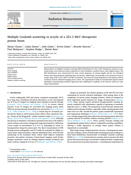
Proton Calibration Technologies in collaboration with the Mayo Proton Clinic and the Arizona State University published the attached paper. Our approach to developing proton Computed Tomography involves using both real and simulated protons. PCT is grateful to Mayo and ASU for their support.
Click here to read the full report:
Proton Calibration Adds COO
Published 2/2025
Proton Computed Tomography Testbed Results Presented at The Latin American Symposium on Nuclear Physics and Applications
Published 7/2024
The initial results from our collaboration with Arizona State University and the Mayo Proton Clinic were presented by Dr. Alarcon, Professor, Department of Physics. The talk was well received. Dr. Alarcon was approached by physicists from CERN and other institutions offering to collaborate with us. The talk demonstrates the viability of our approach to developing proton Computed Tomography (pCT).
Slide 1. The opening slide of the talk

Slide 2, The combination of theory and practice. Excellent agreement between our measurement of the proton beam spread and the beam spread computed by the physics simulation package Geant4.

Slide 3. The conclusions obtained from our experiments, particularly with respect to the validity of our approach to the development of pCT.
Promising Results from Proton CT Tests with Live Beam
Published 11/2023

Researchers from the Arizona State University Physics Department, Proton Calibration Technologies, and the Mayo Clinic Arizona Proton Therapy Center recently conducted experimental tests to characterize the proton energy distribution in the synchrotron beam pulses using scintillation crystal photography.
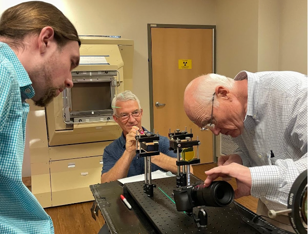
Arizona State University and Proton Calibration Technologies researchers finalize the optical alignment of components in the experimental testbed beamline.
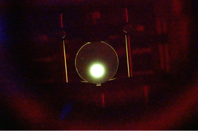
The YAG crystal emits visible photons in proportion to bombardment with 220 MeV protons. Every proton produces some 50 photons at the camera sensor and there are some 10,000,000 per beam pulse. The high intensity spot, 17mm in diameter, indicates a signal strength more than sufficient to proceed with the next set of measurements – sending protons through materials of varying densities. In the next tests a collimating aperture will create one or more mini-beams. Each mini-beam will let us probe the proton relative stopping power of the different phantom materials.
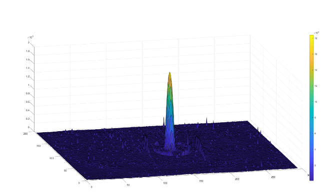
Pictured is a surface map of the light intensity emitted by the scintillation crystal. Notice how sharply the signal stands out with high resolution and excellent signal-to-noise ratio. The steepness of the peak is a good indication of the resolution of mini-beams during the next experimental tests.
Meetings Held to Plan Preliminary Proton CT Experimentation and Testing
Published 5/2023
Paul Mulqueen, CEO of Proton Calibration Technologies and Evgeny Galyaev, CEO of Radiation Detection and Imaging Technologies, met with research team members at a prominent proton therapy center to plan preliminary proton computed tomography testing and experimentation.
Contact
Proton Calibration Technologies
986 N. Cedar Cove Road
Hartselle, AL 35640
